Biplot
- A biplot is a generalization of the simple two-variable Scatterplot
- A biplot overlays a score plot with a loading plot
- This allows displaying information on both samples and variables
- Samples are displayed as points
- while variables are displayed either as
- vectors,
- linear axes
- or nonlinear trajectories
- In the case of categorical variables, category level points may be used to represent the levels of a categorical variable. A generalized biplot displays information on both continuous and categorical variables.
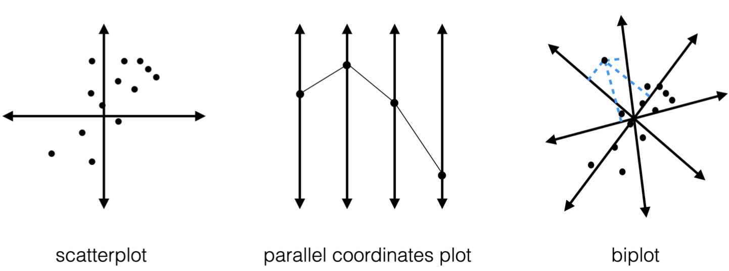
Scatterplot, Parallel Coordinate, and biplot represent three different axis positions.

Loading Plot
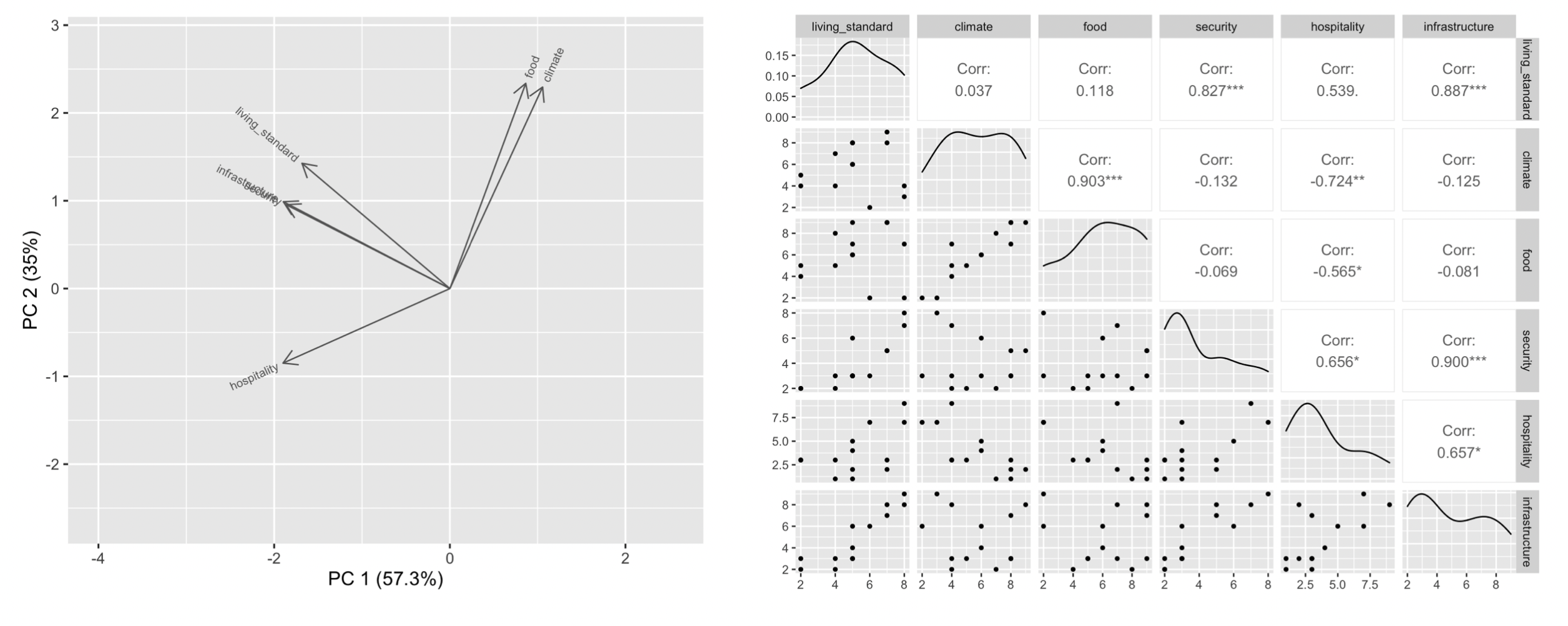
We can use dimension-reduction methods to select or form two main variables, then project other selected/formed variables to the plane (make them linear combinations of the two main variables).
For example, using Principal Components Analysis, we can choose PC1 and PC2 as the two axes, and project original variables to the plane as vectors.

As PCA theory suggests, the first PCs should have wider angles, meaning they have higher variance. Therefore, two vectors with a small angle (or near 180 degrees) have a high correlation; and two vectors that are near perpendicular have a small correlation. We can also compare a loading plot with a Scatterplot Matrix to verify this property.
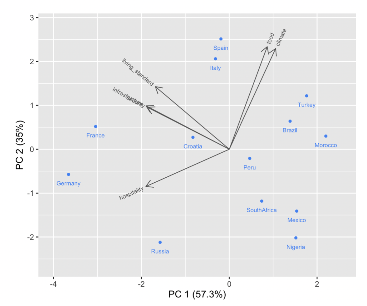
Score Plot
In PCA, transformed data is called PC scores. Similarly, score plots present transformed samples. A biplot combines a loading plot and a score plot.

Elements
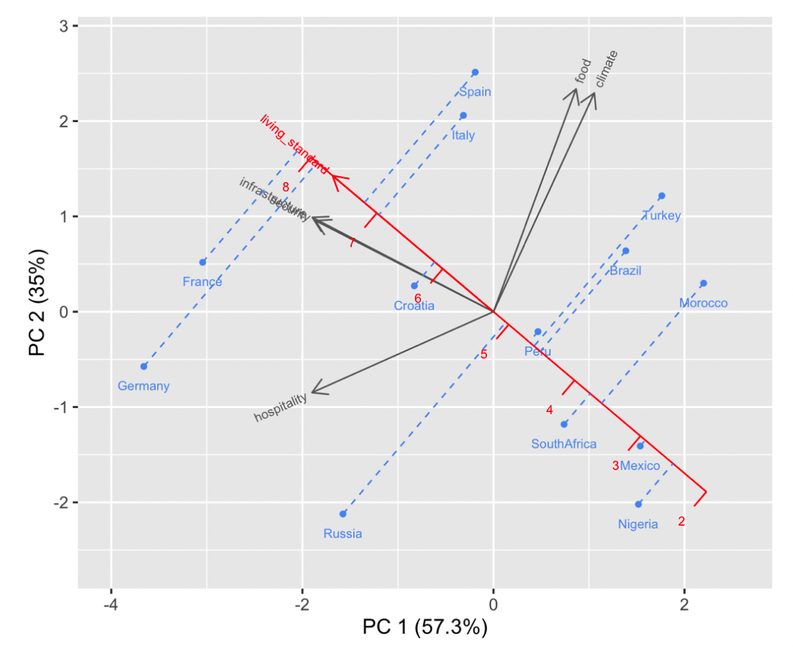
- Calibrated axis
- We can draw ticks on loading vectors
- Projection Lines
- We can project PC scores to vector lines
- to see how samples scale on certain variables

Implementation
- redav
- Install:
remotes::install_github("jtr13/redav") - Use
draw_biplot()- option
key_axisfor calibrated axis and projection lines to it- option
project = FALSEto disable the projection lines
- option
- option
- Install:
 by zcysxy